Multi-Sample Analysis - Wine GC-MS Raw Data

Download sample data and get started using MDC Investigator/Analysis Software.

Step 1: Download Files

1. Download the Wine GC-MS Raw Data from the GitHub repository and unzip it: (On the GitHub page, click the Code drop down and Download ZIP. In your downloads folder, right click on vesi-master.zip and click Extract All...)

   Wine GC-MS Raw Data (Dataset Reference)

2. Download and unzip the example project: (Right click on Wines1DProject.zip and click Extract All...).

   Example Project

Step 2: Import and Process Chromatograms

1. Launch the Project software.

2. From the File menu, select Open Project. Navigate to the location where you unzipped the example project, select the file Wines1D.gcp within the folder, and click Open.

3. Configure the sequence table

   • Expand the Sequences node from the Project Tree on the right side. Select the Seq1 node beneath it.
   • Below the sequence table on the right, click the Edit button.
   • Click the Browse button beside the Data File Path field.
   • Navigate to the location where you unzipped the chromatogram data, select the folder vesi-master\chroms2, and click Open.
   • Click the Done button below the sequence table and Yes to save the changes.
     
     

4. Process the runs

   • From the Run menu, select Auto Process.
   • On the General tab, various parameters for the import are specified.
   

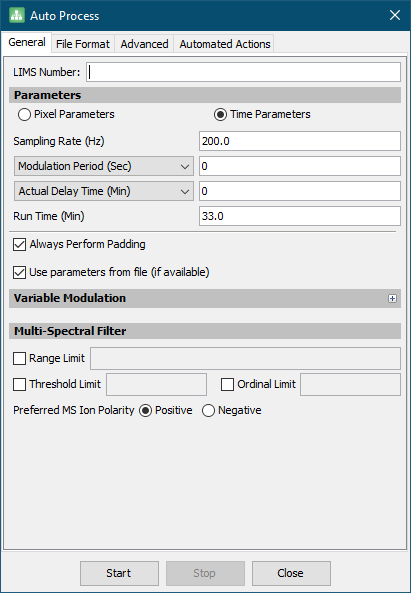
   Tip

   • For importing 1D data, a Modulation Period of 0 should be used.
   • In this example project, most of the values will be read from the provided data files. The modulation period has already been specified in the sequence table and does not need to be set here.

   
   
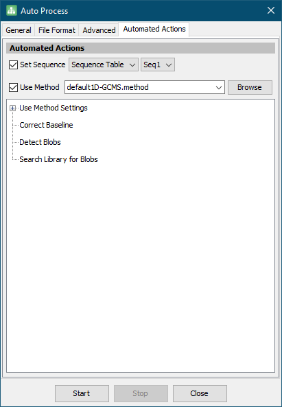
   • On the Automated Actions tab, check the Set Sequence checkbox.
   • Check the Use Method checkbox and select default1D-GCMS.method from the combo box.
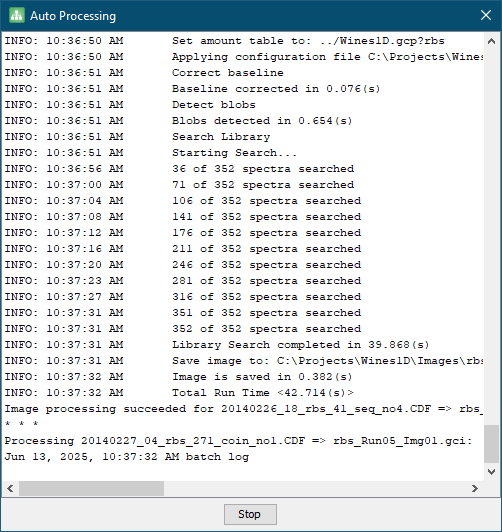
   • Click Start and wait for the data import and processing to complete. This will take some time (about 5-10 minutes).
   • After processing has completed, click Stop and then Close.
   

   

Step 3: Create an Analysis of the Chromatograms

1. From the Run menu, select Investigate Images.

2. Select all images from the Available list and add them to the Selected list. Click OK. Analysis will launch.

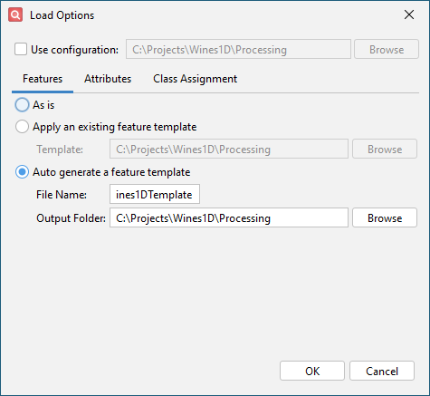
3. Configure settings on the Features tab

   • Click Auto generate a feature template.
   • Enter Wines1DTemplate as the File Name.

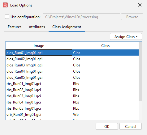
4. Configure settings on the Class Assignment tab

   • Use shift-select to select all clos_Run*.gci files.
   • Click Assign Class and New Label.
   • Enter Clos for the class label and click OK.
   • Repeat this process to assign class Rbs to all rbs_Run*.gci files and Vrb to all vrb_Run*.gci files.
   

   
   
   

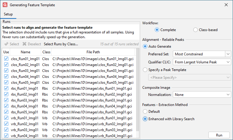
5. Click OK and get the Auto Feature configuration dialog. Enable the Enhanced with Library Search option for Features - Extraction Method.

   

6. Click Run and wait for feature template generation to complete. This will take some time (about 5-10 minutes).

7. Click OK and wait for the data to import.

Step 4: Check Imported Data

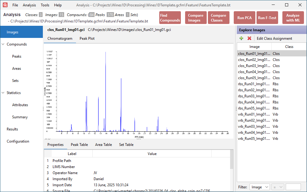
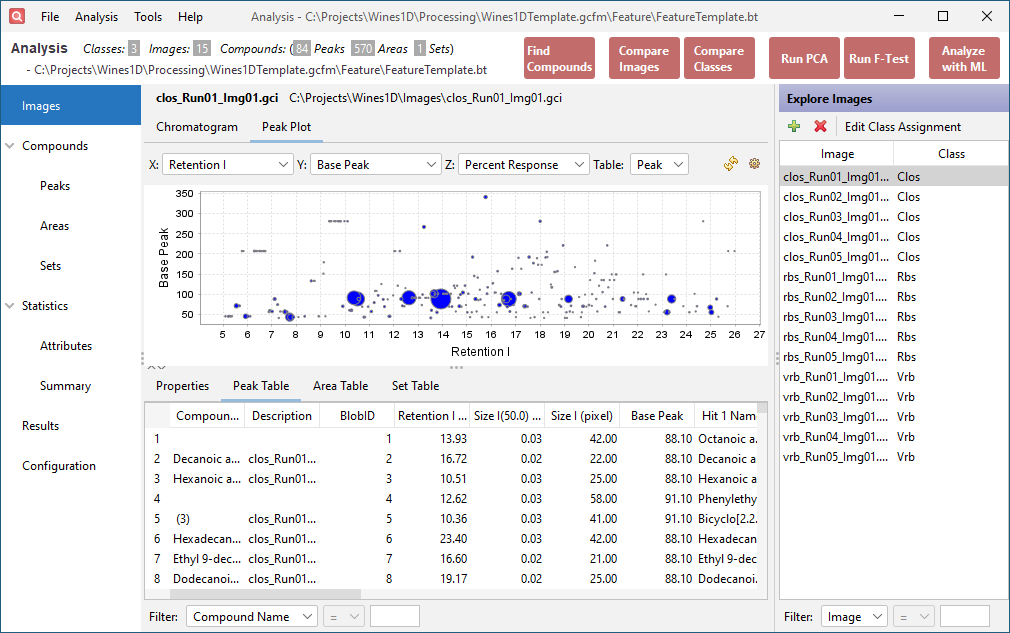
1. The list of imported images is shown on the right side of the window. It lists the image names and associated classes. Select clos_Run01_Img01.gci.

2. Click the Chromatogram tab in the upper half of the window. This displays the source chromatogram.

   

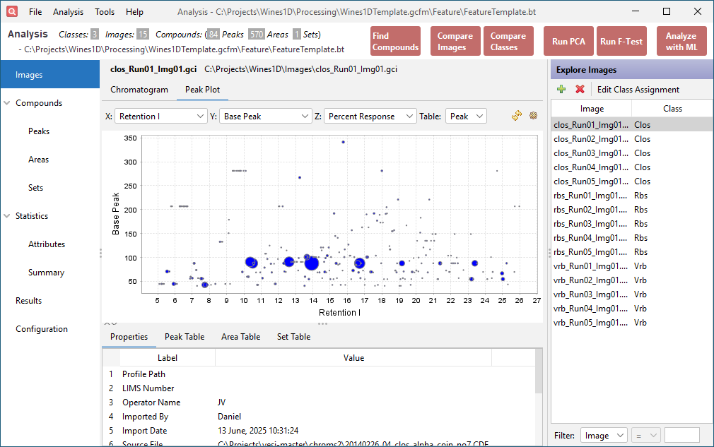
3. Click the Peak Plot tab in the upper half of the window. This displays configurable bubble plots of the data in the Peak Table and Area Table. Set the X axis combo box to Retention I, the Y axis combo box to Base Peak, and the Z axis combo box to Percent Response.

   

4. Click the Peak Table tab in the lower half of the window. This table contains the original data imported from the peak table. The added Description column indicates which feature area the peak belongs to.

   

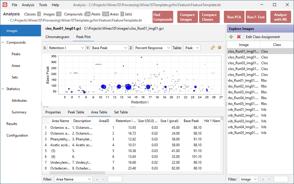
5. Click the Area Table tab in the lower half of the window. This table contains the peak table data restructured to support cross-sample analysis using the computed feature areas. Each row corresponds to a feature area. The values within that row come from the largest peak (by Peak Value) contained in the feature area. The added Description column indicates which peak is reported by the feature area.

   

Step 5: Perform PCA

1. From the action toolbar on the upper-right, click the Run PCA button.

2. On the Configure dialog that appears, select Areas as the Compound Type and Percent Response from the Attribute Selection list. Click OK.

3. Configure the PCA settings with the following:

   • At the bottom of the table, use the Filter to filter the table to the most relevant features. Set the first combo box to F Value, the second combo box to >, and the value field to 5.
   • Click the settings gear button on the upper-right of the PCA chart.
   • Set the Normalization combo box to Normalize by Feature and the Replace missing values with combo box to Zero (0). Click OK.

4. Click the Run PCA button on the upper-right of the PCA chart.